Ingeniero Técnico en Informática de Gestión
Integración Numérica
Trabajo personal 1:-
Utilice las funciones quad y quad8 de MATLAB para hallar:
(a) La integral de exp(-x^2) entre 0 y 2
(b) La integral de exp(-x)*sin(x)/x entre 0 e infinito
(c) Construya a partir del fichero quaddemo.m otro quaddemo1.m que muestre el proceso sobre la integral del apartado (a)
(a) Para ello basta con construir una función de MATLAB, como por ejemplo expo.m, que contenga a la función exp(-x^2) y después aplicar las funciones de matlab quad y quad8 especificando de la manera siguiente los limites de integración.
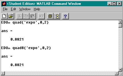
La diferencia entre las funciones quad.m y quad8.m reside en que quad utiliza para calcular la integral una aproximación mediante el método ó regla de Simpson mientras que quad8 hace lo mismo pero utilizando el método de Newton como aproximación.
(b) Para calcular esta integral utilizando quad y quad8, igual que en el apartado primero, es decir definiendo primero la función que nos piden en un fichero aparte que esta vez llamaremos Expsin.m y aplicamos igual que antes quad y quad8, teniendo especial cuidado con los límites de integración ya que esta vez cambian.
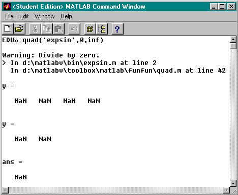
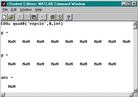
Podemos observar que con ambos procedimientos la solución es NaN, es decir Not a Number.
(c) Para modificar el fichero quaddemo.m hemos de crear una nueva función que llamaremos expo.m en la cual irá implementada la función exp(-x^2).
Con la función quaddemo.m lo que MATLAB realiza es evaluar numéricamente una integral, dicha función llama dentro de ella a la función quad.m la cual realiza la integración utilizando la regla de Simpson.
Nosotros lo que hemos hecho ha sido modificar dicha función adaptándola a nuestro problema, es decir, hemos sustituido la función de demostración Humps.m por la función del apartado (a) y cambiar los limites de integración. Dicha función la hemos denotado por qdemo1.m
expsin.m
function y=expsin(x)
y=(exp(-x).*sin(x))./x
humps.m
function [out1,out2] = humps(x)
%HUMPS A function used by QUADDEMO, ZERODEMO and FPLOTDEMO.
% Y = HUMPS(X) is a function with strong maxima near x = .3
% and x = .9.
%
% [X,Y] = HUMPS(X) also returns X. With no input arguments,
% HUMPS uses X = 0:.05:1.
%
% Example:
% plot(humps)
%
% See QUADDEMO, ZERODEMO and FPLOTDEMO.
% Copyright (c) 1984-98 by The MathWorks, Inc.
% $Revision: 5.4 $ $Date: 1997/11/21 23:26:10 $
if nargin==0, x = 0:.05:1; end
y = 1 ./ ((x-.3).^2 + .01) + 1 ./ ((x-.9).^2 + .04) - 6;
if nargout==2,
out1 = x; out2 = y;
else
out1 = y;
end
Qdemo1.m
%QUADDEMO Demonstrate adaptive numerical quadrature.
% Copyright (c) 1984-98 by The MathWorks, Inc.
% $Revision: 5.3 $ $Date: 1997/11/21 23:26:55 $
echo on
clc
% Quadrature is a technique used to numerically evaluate
% integrals, i.e. to calculate definite integrals. In MATLAB
% a function called QUAD implements quadrature using a
% recursive adaptive Simpson's rule.
% Consider a function called EXPO(x) that we've defined in
% an M-file on disk,
type expo
pause % Strike any key to continue.
% Let's plot this function on the interval from 0 to 1,
fplot('expo',[0,2]')
title('Plot of the function EXPO(x)'), pause
clc
% To integrate this function over the interval 0 < x < 2 we
% invoke QUAD:
% Q = quad('expo',0,2)
pause % Strike any key to start plot of iterations.
clc
% QUAD returns the area under the function.
Q = quad('expo',0,2,1e-4,1);
title(['Area is ',num2str(Q)]),
Q
echo off
disp('End')
Quad.m
function [Q,cnt] = quad(funfcn,a,b,tol,trace,varargin)
%QUAD Numerically evaluate integral, low order method.
% Q = QUAD('F',A,B) approximates the integral of F(X) from A to B to
% within a relative error of 1e-3 using an adaptive recursive
% Simpson's rule. 'F' is a string containing the name of the
% function. Function F must return a vector of output values if given
% a vector of input values. Q = Inf is returned if an excessive
% recursion level is reached, indicating a possibly singular integral.
%
% Q = QUAD('F',A,B,TOL) integrates to a relative error of TOL. Use
% a two element tolerance, TOL = [rel_tol abs_tol], to specify a
% combination of relative and absolute error.
%
% Q = QUAD('F',A,B,TOL,TRACE) integrates to a relative error of TOL and
% for non-zero TRACE traces the function evaluations with a point plot
% of the integrand.
%
% Q = QUAD('F',A,B,TOL,TRACE,P1,P2,...) allows parameters P1, P2, ...
% to be passed directly to function F: G = F(X,P1,P2,...).
% To use default values for TOL or TRACE, you may pass in the empty
% matrix ([]).
%
% See also QUAD8, DBLQUAD.
% C.B. Moler, 3-22-87.
% Copyright (c) 1984-98 by The MathWorks, Inc.
% $Revision: 5.16 $ $Date: 1997/12/02 15:35:23 $
% [Q,cnt] = quad(F,a,b,tol) also returns a function evaluation count.
if nargin < 4, tol = [1.e-3 0]; trace = 0; end
if nargin < 5, trace = 0; end
c = (a + b)/2;
if isempty(tol), tol = [1.e-3 0]; end
if length(tol)==1, tol = [tol 0]; end
if isempty(trace), trace = 0; end
% Top level initialization
x = [a b c a:(b-a)/10:b];
y = feval(funfcn,x,varargin{:});
fa = y(1);
fb = y(2);
fc = y(3);
if trace
lims = [min(x) max(x) min(y) max(y)];
if ~isreal(y)
lims(3) = min(min(real(y)),min(imag(y)));
lims(4) = max(max(real(y)),max(imag(y)));
end
ind = find(~isfinite(lims));
if ~isempty(ind)
[mind,nind] = size(ind);
lims(ind) = 1.e30*(-ones(mind,nind) .^ rem(ind,2));
end
axis(lims);
plot([c b],[fc fb],'.')
hold on
if ~isreal(y)
plot([c b],imag([fc fb]),'+')
end
drawnow
end
lev = 1;
% Adaptive, recursive Simpson's quadrature
if ~isreal(y)
Q0 = 1e30;
else
Q0 = inf;
end
recur_lev_excess = 0;
[Q,cnt,recur_lev_excess] = ...
quadstp(funfcn,a,b,tol,lev,fa,fc,fb,Q0,trace,recur_lev_excess,varargin{:});
cnt = cnt + 3;
if trace
hold off
axis('auto');
end
if (recur_lev_excess > 1)
warning(sprintf('Recursion level limit reached %d times.', ...
recur_lev_excess ))
end
%------------------------------------------------------------
function [Q,cnt,recur_lev_excess] = quadstp(FunFcn,a,b,tol,lev,fa,fc,fb,Q0,trace,recur_lev_excess,varargin)
%QUADSTP Recursive function used by QUAD.
% [Q,cnt] = quadstp(F,a,b,tol,lev,fa,fc,fb,Q0) tries to
% approximate the integral of f(x) from a to b to within a
% relative error of tol. F is a string containing the name
% of f. The remaining arguments are generated by quad or by
% the recursion. lev is the recursion level.
% fa = f(a). fc = f((a+b)/2). fb = f(b).
% Q0 is an approximate value of the integral.
% See also QUAD and QUAD8.
% C.B. Moler, 3-22-87.
LEVMAX = 10;
if lev > LEVMAX
% Print warning the first time the recursion level is exceeded.
if ~recur_lev_excess
warning('Recursion level limit reached in quad. Singularity likely.')
recur_lev_excess = 1;
else
recur_lev_excess = recur_lev_excess + 1;
end
Q = Q0;
cnt = 0;
c = (a + b)/2;
if trace
yc = feval(FunFcn,c,varargin{:});
plot(c,yc,'.');
if ~isreal(yc)
plot(c,imag(yc),'+');
end
drawnow
end
else
% Evaluate function at midpoints of left and right half intervals.
h = b - a;
c = (a + b)/2;
x = [a+h/4, b-h/4];
f = feval(FunFcn,x,varargin{:});
if trace
plot(x,f,'.');
if ~isreal(f)
plot(x,imag(f),'+')
end
drawnow
end
cnt = 2;
% Simpson's rule for half intervals.
Q1 = h*(fa + 4*f(1) + fc)/12;
Q2 = h*(fc + 4*f(2) + fb)/12;
Q = Q1 + Q2;
% Recursively refine approximations.
if abs(Q - Q0) > tol(1)*abs(Q) + tol(2);
[Q1,cnt1,recur_lev_excess] = quadstp(FunFcn,a,c,tol/2,lev+1,fa,f(1),fc,Q1,trace,recur_lev_excess,varargin{:});
[Q2,cnt2,recur_lev_excess] = quadstp(FunFcn,c,b,tol/2,lev+1,fc,f(2),fb,Q2,trace,recur_lev_excess,varargin{:});
Q = Q1 + Q2;
cnt = cnt + cnt1 + cnt2;
end
end
Quaddemo.m
%QUADDEMO Demonstrate adaptive numerical quadrature.
% Copyright (c) 1984-98 by The MathWorks, Inc.
% $Revision: 5.3 $ $Date: 1997/11/21 23:26:55 $
echo on
clc
% Quadrature is a technique used to numerically evaluate
% integrals, i.e. to calculate definite integrals. In MATLAB
% a function called QUAD implements quadrature using a
% recursive adaptive Simpson's rule.
% Consider a function called HUMPS(x) that we've defined in
% an M-file on disk,
type humps
pause % Strike any key to continue.
% Let's plot this function on the interval from 0 to 1,
fplot('humps',[0,1]')
title('Plot of the function HUMPS(x)'), pause
clc
% To integrate this function over the interval 0 < x < 1 we
% invoke QUAD:
% Q = quad('humps',0,1)
pause % Strike any key to start plot of iterations.
clc
% QUAD returns the area under the function.
Q = quad('humps',0,1,1e-3,1);
title(['Area is ',num2str(Q)]),
Q
echo off
disp('End')
quad8.m
function [Q,cnt] = quad8(funfcn,a,b,tol,trace,varargin)
%QUAD8 Numerically evaluate integral, higher order method.
% Q = QUAD8('F',A,B) approximates the integral of F(X) from A to B to
% within a relative error of 1e-3 using an adaptive recursive Newton
% Cotes 8 panel rule. 'F' is a string containing the name of the
% function. The function must return a vector of output values if
% given a vector of input values. Q = Inf is returned if an excessive
% recursion level is reached, indicating a possibly singular integral.
%
% Q = QUAD8('F',A,B,TOL) integrates to a relative error of TOL. Use
% a two element tolerance, TOL = [rel_tol abs_tol], to specify a
% combination of relative and absolute error.
%
% Q = QUAD8('F',A,B,TOL,TRACE) integrates to a relative error of TOL and
% for non-zero TRACE traces the function evaluations with a point plot
% of the integrand.
%
% Q = QUAD8('F',A,B,TOL,TRACE,P1,P2,...) allows coefficients P1, P2, ...
% to be passed directly to function F: G = F(X,P1,P2,...).
% To use default values for TOL or TRACE, you may pass in the empty
% matrix ([]).
%
% See also QUAD, DBLQUAD.
% Cleve Moler, 5-08-88.
% Copyright (c) 1984-96 by The MathWorks, Inc.
% $Revision: 5.13 $ $Date: 1996/10/28 22:15:45 $
% [Q,cnt] = quad8(F,a,b,tol) also returns a function evaluation count.
if nargin < 4, tol = [1.e-3 0]; trace = 0; end
if nargin < 5, trace = 0; end
if isempty(tol), tol = [1.e-3 0]; end
if length(tol)==1, tol = [tol 0]; end
if isempty(trace), trace = 0; end
% QUAD8 usually does better than the default 1e-3.
h = b - a;
% Top level initialization, Newton-Cotes weights
w = [3956 23552 -3712 41984 -18160 41984 -3712 23552 3956]/14175;
x = a + (0:8)*(b-a)/8;
y = feval(funfcn,x,varargin{:});
yllow = min([min(real(y)) min(imag(y))]);
ylhi = max([max(real(y)) max(imag(y))]);
lims = [min(x) max(x) yllow ylhi];
ind = find(~isfinite(lims));
if ~isempty(ind)
[mind,nind] = size(ind);
lims(ind) = 1.e30*(-ones(mind,nind) .^ rem(ind,2));
end
if trace
axis(lims);
% doesn't take care of complex case
plot([a b],[real(y(1)) real(y(9))],'.'), hold on
if ~isreal(y)
plot([a b],[imag(y(1)) imag(y(9))],'+')
end
drawnow
end
lev = 1;
% Adaptive, recursive Newton-Cotes 8 panel quadrature
if ~isreal(y)
Q0 = 1e30;
else
Q0 = inf;
end
[Q,cnt] = quad8stp(funfcn,a,b,tol,lev,w,x,y,Q0,trace,varargin{:});
cnt = cnt + 9;
if trace
hold off
axis('auto');
end
%------------------------------------------------------------------
function [Q,cnt] = quad8stp(FunFcn,a,b,tol,lev,w,x0,f0,Q0,trace,varargin)
%QUAD8STP Recursive function used by QUAD8.
% [Q,cnt] = quad8stp(F,a,b,tol,lev,w,f,Q0) tries to approximate
% the integral of f(x) from a to b to within a relative error of tol.
% F is a string containing the name of f. The remaining arguments are
% generated by quad8 or by the recursion. lev is the recursion level.
% w is the weights in the 8 panel Newton Cotes formula.
% x0 is a vector of 9 equally spaced abscissa is the interval.
% f0 is a vector of the 9 function values at x.
% Q0 is an approximate value of the integral.
% See also QUAD8 and QUAD.
% Cleve Moler, 5-08-88.
LEVMAX = 10;
% Evaluate function at midpoints of left and right half intervals.
x = zeros(1,17);
f = zeros(1,17);
x(1:2:17) = x0;
f(1:2:17) = f0;
x(2:2:16) = (x0(1:8) + x0(2:9))/2;
f(2:2:16) = feval(FunFcn,x(2:2:16),varargin{:});
if trace
plot(x(2:2:16),f(2:2:16),'.');
if ~isreal(f)
plot(x(2:2:16),imag(f(2:2:16)),'+');
end
drawnow
end
cnt = 8;
% Integrate over half intervals.
h = (b-a)/16;
Q1 = h*w*f(1:9).';
Q2 = h*w*f(9:17).';
Q = Q1 + Q2;
% Recursively refine approximations.
if (abs(Q - Q0) > tol(1)*abs(Q)+tol(2)) & (lev <= LEVMAX)
c = (a+b)/2;
[Q1,cnt1] = quad8stp(FunFcn,a,c,tol/2,lev+1,w,x(1:9),f(1:9),Q1,trace,varargin{:});
[Q2,cnt2] = quad8stp(FunFcn,c,b,tol/2,lev+1,w,x(9:17),f(9:17),Q2,trace,varargin{:});
Q = Q1 + Q2;
cnt = cnt + cnt1 + cnt2;
end
Descargar
| Enviado por: | Tyler |
| Idioma: | castellano |
| País: | España |
Todos los derechos reservados.